Linearized relative motion of a secondary spacecraft about a primary in a circular orbit (Curtis chapter 7).
Linearization
- Primary (reference orbit) and secondary (possibly thrusting):
- Relative position and its inertial acceleration:
- Assumption: , with
- Expand the term:
- binomial expansion :
- (the notes write the remaining terms of , , on the end of this line; they are combined in the next step)
- Keep first-order terms in :
- Components of in the RSW frame of :
, with radial (so ):
Rotating Frame
- The RSW frame rotates, so (transport theorem):
- = orbital angular velocity of the primary:
- For circular motion this is a constant, equal to the mean motion times the unit vector
- The tangential acceleration is then 0
- For the other two terms, expand in components:
- and the gravity term, with :
- Altogether:
HCW Equations
Hill-Clohessy-Wiltshire (HCW) Equations
- radial, along-track, cross-track; : components of
- Linear, constant coefficients (circular reference orbit)
Solving the HCW Equations
- Assume no external forces:
- The one-dimensional equation is decoupled from the rest (simple harmonic motion):
- Two coupled - equations in the orbital plane; differentiate the equation and substitute
:
- With :
- Match initial conditions:
Corrected from the notes
- The handwriting writes (double dot on )
- From the equation at , , so it is ; the following and the typed solution on the next page both use
- So:
- Then from :
Secular drift
- The secular term grows without bound
- This secular term arises only because of the linearization approximation, which is violated given enough time
- It vanishes when
Full Solution
State Transition Matrix
- These equations can be written as sub-matrices of the
state transition matrix:
Example Trajectories
- Curtis Fig. 7.6: trajectory of relative to in the comoving frame during five of the target’s orbits, target eccentricity 0.1: loops that drift steadily along (about 40 km over five orbits)
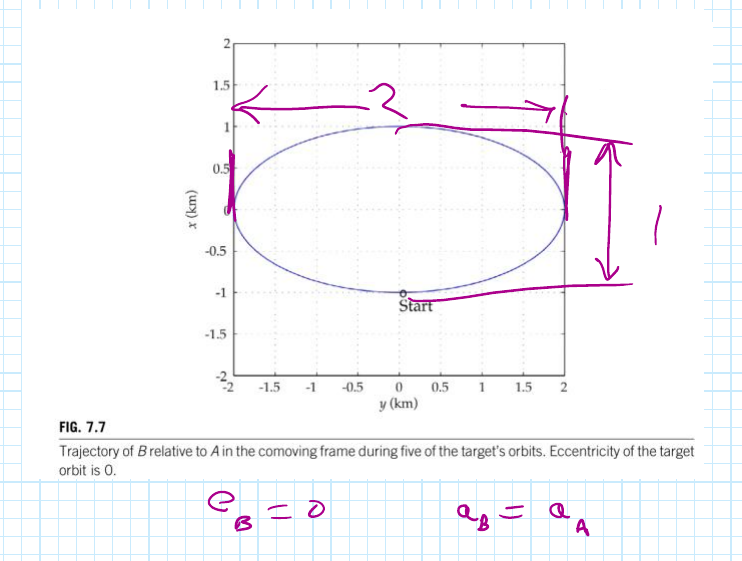
- Curtis Fig. 7.7: same, target eccentricity 0: a closed ellipse, 2 (along-track) by 1 (radial), annotated ,
- Same semimajor axis same period no drift
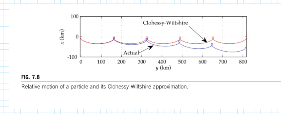
- Curtis Fig. 7.8: the actual relative motion slowly departs from the Clohessy-Wiltshire prediction over hundreds of km: the linearization breaks down