Linearizing a nonlinear state-space model about a known reference solution, producing a linear model for the deviations from that reference.
Taylor Series Approximation
- Why use in the pendulum example? Recall:
- and for , , etc. (H.O.T. negligible)
- Via Taylor we can do a similar expansion for most functions, around arbitrary reference points (other than 0):
- so for small :
- Similarly, if depends on two (or more) variables:
- And we can do this with each function that appears in our problem (; )
Reference Solution
- Assume we know a solution for the state eq’n given IC and input , i.e.
- Any other solution must also satisfy
- Differencing:
- By Taylor:
Jacobian Matrices
- are the Jacobian matrices:
- where means the derivatives are evaluated for the reference conditions
- i.e. using , , after taking the indicated derivatives
Linearized Deviation Model
Linearized State Equation
- Finally, we can write a model for the deviations of the state vector from the assumed reference:
- where
- Jacobians of
- and
- Finally, has the H.O.T., so that is small when and are small
Important note
- i.e. linearized stability the full solution converges back to the reference solution (not to !!)
- Also remember is not the physical input . It is the deviation of from the reference input that gives rise to the reference solution used in the linearization
Example: Pendulum Jacobians
Pendulum Linearization
- From the pendulum model:
- Jacobians:
- The bottom row depends on the specific reference solution!
- If the reference solution is , , (pendulum is nominally motionless, straight down), then
- which agrees with the previous hand-waving analysis (, )
- Note = slope of the friction curve at 0
Aside: friction modeling
- Friction is notoriously difficult to model accurately
- It is dissipative, so , but it can contain discontinuities:
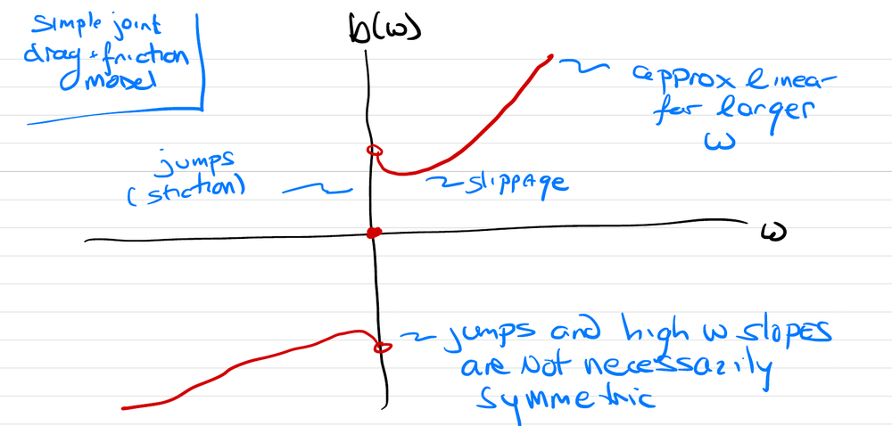
- Jumps at (stiction), followed by slippage; approximately linear for larger
- Jumps and high- slopes are not necessarily symmetric
- Such a function cannot be completely treated within the formalism above, since it fails to be differentiable at 0
Output Linearization
- We can similarly linearize the output eq’n for any reference solution. Let
- where (reference output)
- Then
- where
- and has H.O.T. which are negligible if and are small
Note again
- is the deviation of the output from the reference, not the physical output
Pendulum About an Arbitrary Reference
Pendulum Linearization, General Reference Solution
- Pendulum:
- Linearization has
- and
- where
- Suppose the output is :
- The equivalent I/O DE for the linearized output satisfies
- Do the properties of this DE change for different reference solutions? If so, how? see Linearized Dynamics at Different Equilibria