How a (possibly nonlinear) physical model is packaged as a state equation plus an output equation. Symbols follow Prof. Sanner’s notation: physical state , physical input , physical output .
State of a System
- The state of a system is a collection of quantities such that knowledge of these quantities at a single time , together with knowledge of the inputs , , is sufficient to predict the outputs
- Block diagram: input [system, with internal state ] output
- The state defines a mapping:
- A feasible mapping must make this constructive
- State vector of the system:
State Equation
Implicit Form
- Assume physical modeling specifies the rate of change of the chosen states via implicit DEs of the form:
- ( equations)
- i.e. the rate of change of each potentially depends on the instantaneous values of the states, the state derivatives, the inputs, and time itself ( variables)
- More compactly:
- Even more compactly, stack them into a vector of functions:
State Equation
- is the state equation for the system
Explicit Form
- Common alternate form is the explicit form:
- But this can be an unnecessarily restrictive assumption in some cases
Linear State Equations
- The state equation is linear iff:
Standard Form
- If the state eq’n is linear, with invertible matrix , then
- can be re-written as the “standard form” for a linear state eq’n:
NOTE
- will be invertible in all examples considered in this class
Output Equation
- Block diagram: () [system, ()] ()
- Full model:
- Like the state eq’n, the output eq’n is linear iff:
- The system is linear if both the state and output eq’ns are
Example: Simple Pendulum
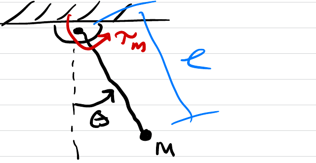
Simple Pendulum Model
- Take states:
- Physics:
- : friction, drag
- : applied torque (servo motor) this is the input,
- Equivalently:
- Rewrite in implicit form:
- Note that this is not linear, b/c of the term, and b/c is not explicitly specified
- However, if we assume , (linear friction), then the state eq’n is linear with:
- Note: constant eq’n is also time invariant
- Output: suppose we want to control the angle . Then
- (linear and time-invariant here)
- Why is justified? See Linearization