“Geometric” (Lyapunov) stability analysis: deduce stability from how a size measure of changes, without knowing .
Rate of Change of the Norm
- How do we deduce whether has the stability properties if we don’t know exactly what looks like?
- We could equivalently think in terms of the change in over time, i.e.
- (in fact with , so perhaps more restrictive than necessary…)
- or
- With the homogeneous dynamics :
A First Stability Test
- “Geometric” stability analysis (Lyapunov): examine the behavior of via different metrics
- [Initially homogeneous / “internal” stability]
- For example:
- which is a quadratic form
- With (symmetric), the Rayleigh-Ritz inequality gives
- if the system is stable i.s.L.
Theorem
- If
- then the system is stable i.s.L.
Careful
- This does not mean that implies instability!
- It might, or might not requires further investigation
Re-Interpreting the Result
- (Previous result, re-interpreted.) We have shown
- where
- So that if
- i.e. if is positive semi-definite. Equivalently
Too restrictive
- is too restrictive to fully characterize stability
- Sketch of vs. , both starting from :
- a blue curve that only decreases ()
- a red curve that first rises well above , with bumps, and then decays: the red one is also stable, but doesn’t satisfy
- reinterpret the argument more geometrically
Level Sets and Invariant Sets
- Let
- Note that:
- The “level sets” for define a nested family of closed contours
- Rate of change along solutions:
- :
- points into the contour (or at worst along the boundary)
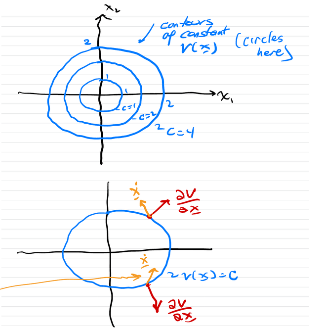
- motion at any point on any contour is directed to the interior of that contour
Invariant Sets
- This means that the interior of each contour,
- defines an “invariant set”, i.e. if such that , then necessarily
- means each contour is an invariant set, and the state can never “escape” the contour it starts inside stability i.s.L.
NOTE
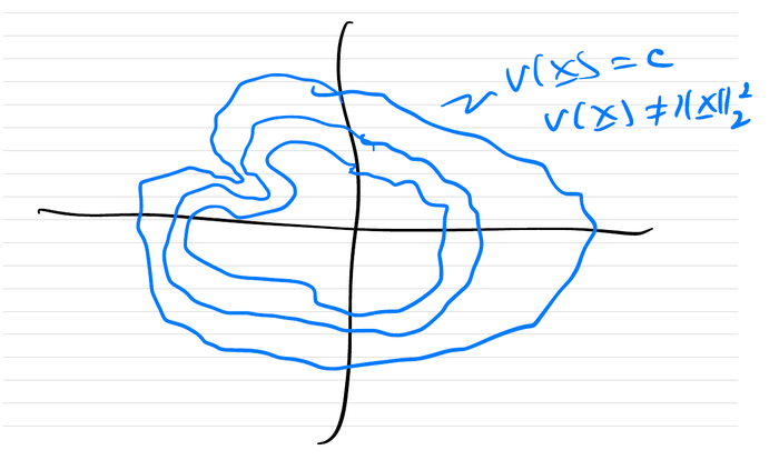
- Nothing in these arguments requires circular contours! Any nested set of closed contours works
Quadratic Lyapunov Functions
- For linear systems, we need only consider for which the level sets are elliptical, which can be described using the quadratic form
- (nested ellipses )
- Terminology:
- A general satisfying the nested contour requirement above is known as a “Lyapunov function”
- A quadratic form for is known as a quadratic Lyapunov function (QLF)
- Note that our original with
- Allowing time-varying leads to the Lyapunov Equation