Modal Decomposition

Reading the LTI response , mode by mode, using the right eigenvectors , left eigenvectors and eigenvalues of (distinct eigenvalues; see Dyadic Expansion).

Homogeneous Response

• Example application #2 of the dyadic expansion: solving the homogeneous eq’n
• We know . Use the dyadic expansion:
  • (the are dot products!)

Modal Form of the Homogeneous Response

• : the “modes” of the state eq’n
• : amount of the mode present in the response (constant) = the extent the mode is “excited” by the ICs
  • : dot product of the left eigenvector with the ICs
• : right eigenvectors of ; : left eigenvectors of ; : eigenvalues of ; : initial conditions

Initial Condition Along an Eigenvector

• Suppose, for example,
  • (i.e. the IC lies along one of the right eigenvectors)
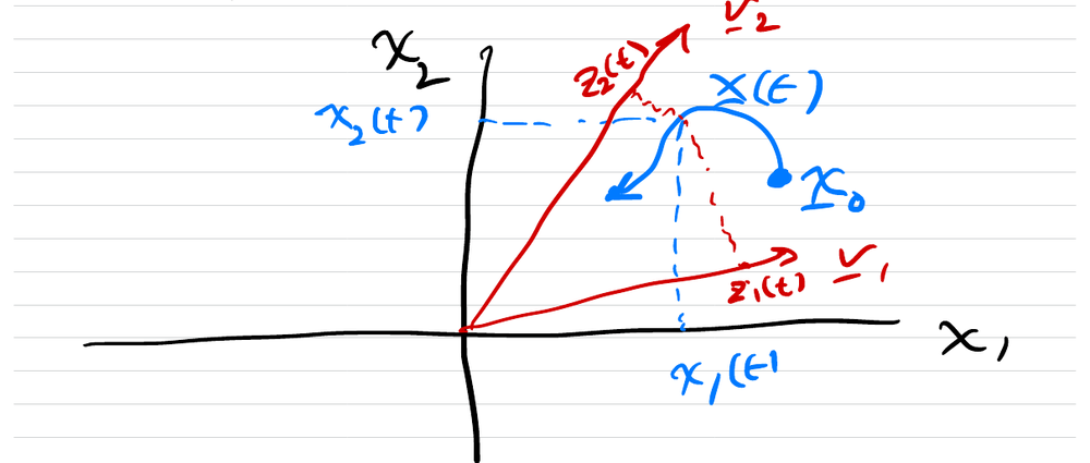
  • Sketch: in the - plane with eigenvectors , the IC sits on the line and moves straight along that line
• Then, by bi-orthonormality:
• Only the mode is present in the response! (No other modes contribute to for such an IC)

Forced Response

• Forced solutions:
• Column partition :
  • describes how the input affects the rate of change of
  • see this more explicitly in the solutions for :
• • (: dot product again!)
• Hence
  • where
  • Each term of the sum: amount of the mode due to input
  • : “strength” of the impact of the input on the mode
• the input has no impact on the mode

Output Response

• Row partition:
• Then for :
  • : how much of the mode is “visible” in the output
• If the mode is not visible in the output

Modal Coordinates

• Let in the above eq’ns. Then
  1. Expansion:
     • : coordinates of in the basis given by
  2. and
• so that

Decoupled Modal Dynamics

• Decoupled!!

• Laplace:
  • and
  • the TFM in partial-fraction form

Modal Basis

• • expresses the solution in a new basis, given by the eigenvectors of
• This is sometimes called the “modal basis” and the “modal coordinates”:
• 

Modal Form

• Then
• Output:

Modal Form of System Dynamics

• Block diagram: [system, or ]
  • The internal details are different, but and are the same in both models same input/output behavior
• There is nothing special about the eigenvector matrix here: see State Coordinate Transformations

Complex Eigenvalues: Block Modal Form

• The modal coordinate transform results in the decoupled
• We might want to modify this if is complex, since then the solutions are also complex and hard to interpret physically

Block Modal Form

• Suppose
• There exists a nonsingular such that
  • the “block modal form” (zeros off the blocks)
  • Pure diagonalization would instead give
• • ; (so only , are needed)
• Then
  • (using the rotation-like and block-diagonal forms)
• and
  • Oscillations for the 1st complex mode occur in a plane spanned by
  • Oscillations for the 2nd complex mode occur in the plane spanned by

Possible slip in notes

• The notes write the second eigenvalue as before noting ; written here as

Exciting a Single Oscillatory Mode

• Suppose
• Then
• • only the 1st mode is present, and creates changes in in only 2 directions:
• Note that
• Thus, if , then
  1. The solution contains only the 1st mode (oscillations with frequency )
  2. for all
  • i.e. the modal oscillations occur in a planar subset of the original state space
• Similarly would uniquely excite the 2nd oscillatory mode, and the resulting would be confined to this planar subset of state space

Polar Visualization

• An alternate visualization: let the complex eigenvector be expressed in polar form:
• For a mode with such an eigenvector, the corresponding oscillations in each component of will have relative amplitude and relative phase
  • i.e. the ratio of the amplitude of oscillations in compared to the amplitude of oscillations in would be
  • and the difference in phase between oscillations in and would be
• Another reason to find an alternate for LTI: repeated (real) eigenvalues Jordan Normal Form