The unique matrix that maps the state at one time to the state at another for .
Definition
- From the fundamental matrix, every homogeneous solution is , where . Thus
State Transition Matrix
- is the “state transition matrix” (STM) for the system: unique to the system (any choice of fundamental matrix gives the same )
- With the STM, the general solution of the state eq’n is
- if we know (or ) we know everything about the system. What can we say about these generally?
- is an matrix, defined by functions of
- Usually we will not know these functions exactly, and must argue using only generic properties of any STM
Properties of Any STM
- for any
- is nonsingular for any
- But we know (Lemma 2), and the same proof shows at any finite
- Inverse:
- Pf:
- Derivatives:
- Pf a):
- Pf b) (using the derivative of the inverse, ):
- For any :
- the “composition” or “semi-group” property
- Pf:
Composition, Intuitively
- Consider the homogeneous solution (with ), :
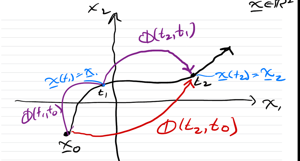
- Note also this implies
Constructing the STM
- Can we actually constructively determine the STM for an arbitrary ? i.e. find the functions of
- Generally no, but we can try:
- Find a family of fundamental solutions
- remember
- Numerically solve for on a grid of points
- Brute force series expansion (may possibly simplify): the “Peano-Baker” series
- Find a family of fundamental solutions
Peano-Baker Series
- IF
- (i.e. commutes with its integral) for every
- THEN
- Recall the scalar exponential function satisfies
- By analogy the above power series defines the matrix exponential function. Common to write (when the commutativity condition is satisfied!):
- where by “exp” is meant the formal power series above
- This looks comfortingly familiar, but we must be careful: see Matrix Exponential
Constant A
- As a final possible simplification, if is constant, then the commutativity condition is definitely satisfied, and
- (Note: can also write when is understood to be constant)
Other Results Involving the STM
- Under a change of state coordinates : (proof)
- For periodic , the STM factors into a periodic part and an LTI part: Floquet Theory